An Exploratory Data Analysis on how countries’ Digital Skills Indicator scores in 2023 compare to their performance in 2021.
data analysis
data visualization
eurostat
digital skills indicator
Author
Cozmina Secula
Published
September 12, 2024
Translate Widget
In the second part of this Exploratory Data Analysis (EDA), I will explore how countries’ DSI scores in 2023 compare to their performance in 2021. In the first part, I introduced the data set, provided an overview of composite indicators, introduced the DSI, analyzed its components, and shared key insights from the analysis.
The key questions guiding this analysis are:
What does the distribution of DSI scores in 2023 look like compared to 2021?
How has each country’s DSI score changed from 2021 to 2023?
What does the distribution of DSI scores in 2023 look like compared to 2021?
Summary Statistics
Show the code
digital_skills_summary<-raw_data|># Keep only "at least basic skills" for Overall Digital Skills filter(!indicator%in%c("Individuals with above basic overall digital skills (all five component indicators are at above basic level)","Individuals with basic overall digital skills (all five component indicators are at basic or above basic level, without being all above basic)"))|># Extract `digital skills` and `indicator level` from the `indicator` columnmutate( digital_skills =case_when(str_detect(indicator, "communication and collaboration")~"Communication and Collaboration Skills",str_detect(indicator, "digital content creation")~"Digital Content Creation Skills",str_detect(indicator, "information and data literacy")~"Information and Data Literacy Skills",str_detect(indicator, "overall digital skills")~"Overall Digital Skills",str_detect(indicator, "problem solving skills")~"Problem Solving Skills",str_detect(indicator, "safety skills")~"Safety Skills"), indicator_level =case_when(# Special case for overall digital skills with at least basic levelstr_detect(indicator, "basic overall digital skills \\(all five component indicators are at basic or above basic level\\)")~"At least basic skills",# General casesstr_detect(indicator, "basic or above basic")~"Basic or above basic skills",str_detect(indicator, "above basic")~"Above basic skills",str_detect(indicator, "basic")~"Basic skills"))# Pivot Data (I)country_codes<-data.frame( Country =c("Austria", "Belgium", "Bulgaria", "Croatia", "Cyprus", "Czechia", "Denmark", "Estonia", "Finland", "France", "Germany", "Greece", "Hungary", "Ireland", "Italy", "Latvia", "Lithuania", "Luxembourg", "Malta", "Netherlands", "Poland", "Portugal", "Romania", "Slovakia", "Slovenia", "Spain", "Sweden", "EU_27"), ISO_Code =c("AT", "BE", "BG", "HR", "CY", "CZ", "DK", "EE", "FI", "FR", "DE", "GR", "HU", "IE", "IT", "LV", "LT", "LU", "MT", "NL", "PL", "PT", "RO", "SK", "SI", "ES", "SE", "EU"))dsi<-digital_skills_summary|>filter(digital_skills=="Overall Digital Skills")|>select(year, country, value)|>pivot_wider(names_from =year, values_from =value)|>rename( `2021` =`2021`, `2023` =`2023`, Country =country)|>mutate(Change =`2023`-`2021`, `2021` =round(`2021`, 1), `2023` =round(`2023`, 1))|>left_join(country_codes, by =c("Country"="Country"))# Pivot Longerdsi_longer<-dsi|>pivot_longer(cols =`2021`:`2023`, names_to ="year", values_to ="value")|>select(Country, year, value)dsi_longer_summary<-dsi_longer|>filter(Country!="EU")|>group_by(year)|>summarise( count =n(), mean =round(mean(value, na.rm =TRUE), 2), median =round(median(value, na.rm =TRUE), 2), minimum =min(value, na.rm =TRUE), maximum =max(value, na.rm =TRUE), std_dev =round(sd(value, na.rm =TRUE),2), iqr =round(IQR(value, na.rm =TRUE),2))dsi_longer_summary|>kbl(caption ="Summary Statistics")|>kable_classic(full_width =F, html_font ="Palatino linotype")
Summary Statistics
year
count
mean
median
minimum
maximum
std_dev
iqr
2021
28
56.21
55.25
27.8
79.2
11.89
13.95
2023
28
57.55
58.95
27.7
82.7
12.42
14.23
Visualizing Distribution
Show the code
year_color<-c(`2021` ="#33645FB3", `2023` ="#9D1B1FB3")# Function to find the first two and last two values find_first_last<-function(df){df|>group_by(year)|>arrange(value)|>slice(c(1:2, (n()-1):n()))|>select(Country, year, value)}# Function to label specific countrieslabel_specific_countries<-function(df, country_list){df|>filter(Country%in%country_list)|>select(Country, year, value)}# Find first two and last two values first_last<-find_first_last(dsi_longer)ggplot(dsi_longer,aes(x =value, y =year, color =year))+geom_quasirandom(orientation =NULL, varwidth =TRUE, dodge.width =0.75)+stat_summary(aes(group =year), fun =median, fun.min =median, fun.max =median, geom ="crossbar", color ="black", width =0.7, lwd =0.2, position =position_dodge(width =0.75))+# Label the first two and last two by valuegeom_text_repel(data =first_last, aes(label =Country), nudge_x =0.1, direction ="y", hjust =0.3, vjust =1, family ="Palatino linotype", size =4.5)+scale_x_continuous(labels =scales::percent_format(scale =1), limits =c(20, 100), breaks =seq(20, 100, by =20))+theme_minimal()+labs( title =glue::glue("Distribution of Digital Skills <br>(at least basic skills)"), subtitle =glue::glue("<span style='color:#9D1B1FB3'><b>2023</b></span> compared to <span style='color:#33645FB3'><b>2021</b></span>"), x ="% of individuals")+scale_color_manual(values =year_color)+theme( panel.grid.minor.x =element_blank(), axis.title.y =element_blank(), axis.text.y =element_blank(), axis.text.x =element_text(color ="#646369", family ="Palatino linotype", size =12), axis.title.x =element_text(hjust =0, color ="#646369", family ="Palatino linotype", size =14), legend.position ="none", plot.title =element_markdown(color ="#414040", size =24, family ="Palatino linotype", face ="bold", margin =margin(0, 0, 12, 0)), plot.title.position ="plot", plot.subtitle =element_textbox_simple(size =20, vjust =1, margin =margin(0, 0, 12, 0), color ="#646369", family ="Palatino linotype"))+geom_richtext(aes(x =59, y =2.55, label ="Median: 58.95 %"), family ="Palatino linotype", size =4.5, lineheight =1.2, color ="#414040", hjust =0, vjust =1.03, label.color =NA, fill =NA)+geom_richtext(aes(x =54.5, y =1.56, label ="Median: 55.25 %"), family ="Palatino linotype", size =4.5, lineheight =1.2, color ="#414040", hjust =0, vjust =1.03, label.color =NA, fill =NA)
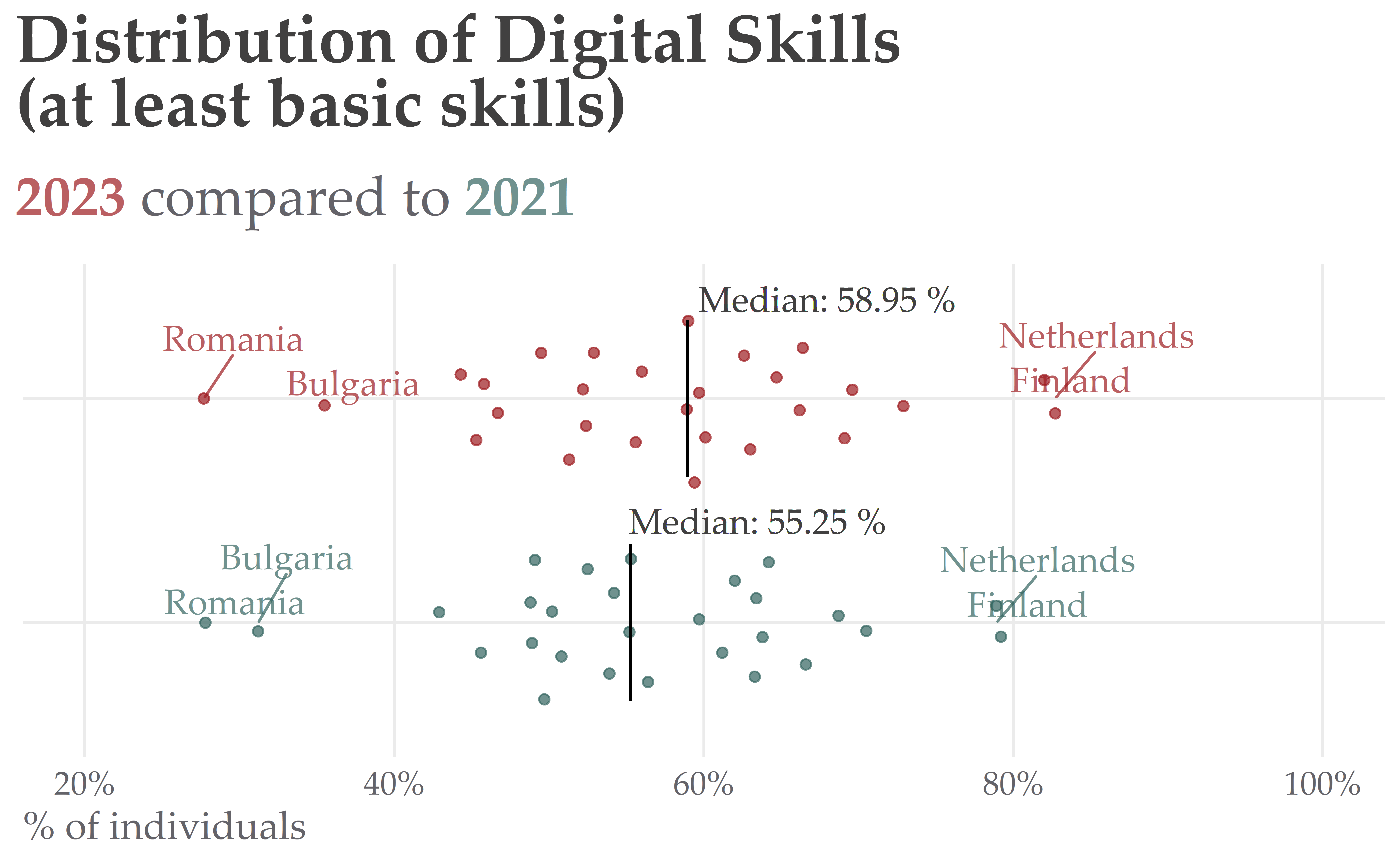
The chart presents the distribution of digital skills (at least basic skills) for 2023 compared to 2021 across EU countries. The data is divided into two groups, with 2023 represented in red and 2021 in green.
Main observations:
The median percentage of individuals with at least basic digital skills increased from 55.25% in 2021 to 58.95% in 2023. This indicates a general improvement in digital skill levels across the surveyed countries.
Finland and the Netherlands consistently stand out with the highest percentages of individuals with basic digital skills in both 2021 and 2023. This shows that these countries have maintained their digital skills advantage.
On the other hand, Romania and Bulgaria have the lowest percentages of individuals with basic digital skills in both years. While Bulgaria shows some improvement in 2023, Romania remains stagnant at its 2021 level.
Both years show a relatively even spread of countries around the 50%–70% range. This suggests that most countries are gradually converging towards having most individuals with at least basic digital skills, although the rate of improvement varies.
Overall, the graph shows an encouraging trend towards higher digital skills levels in 2023 compared to 2021, with a notable improvement in the median. However, the digital divide remains, as evidenced by the extremes: countries like Finland and the Netherlands are leading, while Romania and Bulgaria continue to lag behind. The data suggest a general trend of incremental improvements in at least basic digital skills across most countries.
How has each country’s DSI score changed from 2021 to 2023?
Show the code
# Bar chart function for percentage pointsbar_chart_pos_neg<-function(label, value, max_value=1, height="1rem",pos_fill="#33645FFF", neg_fill="#9D1B1FFF"){neg_chart<-div(style =list(flex ="1 1 0"))pos_chart<-div(style =list(flex ="1 1 0"))width<-paste0(abs(value/max_value)*100, "%")if(value<0){bar<-div(style =list(marginLeft ="0.5rem", background =neg_fill, width =width, height =height))chart<-div( style =list(display ="flex", alignItems ="center", justifyContent ="flex-end"),label,bar)neg_chart<-tagAppendChild(neg_chart, chart)}else{bar<-div(style =list(marginRight ="0.5rem", background =pos_fill, width =width, height =height))chart<-div( style =list(display ="flex", alignItems ="center"),bar, label)pos_chart<-tagAppendChild(pos_chart, chart)}div(style =list(display ="flex"), neg_chart, pos_chart)}# Define the maximum value for scaling (use absolute maximum from relevant columns)max_change<-max(abs(dsi$Change))# Define composite indicator columnscomposite_indicator_cols<-c("2021", "2023", "Change")# Function to generate a color based on the score (percentage)get_score_color<-function(score, min_score=0, max_score=100){# Blue palette transitionblue_pal<-function(x)rgb(colorRamp(c("#77BAB2","#33655F"))(x), maxColorValue =255)# Normalize the score to the range [0, 1]normalized<-(score-min_score)/(max_score-min_score)# Return the color for the normalized scoreblue_pal(normalized)}# Function to generate the donut chart with a colordonut_chart<-function(value, color){# All units are in rem for relative scalingradius<-1.5diameter<-3.75center<-diameter/2width<-0.25slice_length<-2*pi*radiusslice_offset<-slice_length*(1-value/100)# Generate SVG donut chartdonut_chart<-paste0('<svg width="', diameter, 'rem" height="', diameter, 'rem" style="transform: rotate(-90deg);" focusable="false">','<circle cx="', center, 'rem" cy="', center, 'rem" r="', radius, 'rem" fill="none" stroke-width="', width, 'rem" stroke="rgba(0,0,0,0.1)"></circle>','<circle cx="', center, 'rem" cy="', center, 'rem" r="', radius, 'rem" fill="none" stroke-width="', width, 'rem" stroke="', color, '"',' stroke-dasharray="', slice_length, 'rem" stroke-dashoffset="', slice_offset, 'rem"></circle>','</svg>')# Label in the centerlabel<-paste0('<div style="position: absolute; top: 50%; left: 50%; transform: translate(-50%, -50%)">',value, '%</div>')# Final donut chart HTMLpaste0('<div style="display: inline-flex; position: relative; width: ', diameter, 'rem; height: ', diameter, 'rem;">', donut_chart, label, '</div>')}# Define a mapping from ISO codes to the flag URLsflag_urls<-list("AT"="https://hatscripts.github.io/circle-flags/flags/at.svg","BE"="https://hatscripts.github.io/circle-flags/flags/be.svg","BG"="https://hatscripts.github.io/circle-flags/flags/bg.svg","HR"="https://hatscripts.github.io/circle-flags/flags/hr.svg","CY"="https://hatscripts.github.io/circle-flags/flags/cy.svg","CZ"="https://hatscripts.github.io/circle-flags/flags/cz.svg","DK"="https://hatscripts.github.io/circle-flags/flags/dk.svg","EE"="https://hatscripts.github.io/circle-flags/flags/ee.svg","FI"="https://hatscripts.github.io/circle-flags/flags/fi.svg","FR"="https://hatscripts.github.io/circle-flags/flags/fr.svg","DE"="https://hatscripts.github.io/circle-flags/flags/de.svg","GR"="https://hatscripts.github.io/circle-flags/flags/gr.svg","HU"="https://hatscripts.github.io/circle-flags/flags/hu.svg","IE"="https://hatscripts.github.io/circle-flags/flags/ie.svg","IT"="https://hatscripts.github.io/circle-flags/flags/it.svg","LV"="https://hatscripts.github.io/circle-flags/flags/lv.svg","LT"="https://hatscripts.github.io/circle-flags/flags/lt.svg","LU"="https://hatscripts.github.io/circle-flags/flags/lu.svg","MT"="https://hatscripts.github.io/circle-flags/flags/mt.svg","NL"="https://hatscripts.github.io/circle-flags/flags/nl.svg","PL"="https://hatscripts.github.io/circle-flags/flags/pl.svg","PT"="https://hatscripts.github.io/circle-flags/flags/pt.svg","RO"="https://hatscripts.github.io/circle-flags/flags/ro.svg","SK"="https://hatscripts.github.io/circle-flags/flags/sk.svg","SI"="https://hatscripts.github.io/circle-flags/flags/si.svg","ES"="https://hatscripts.github.io/circle-flags/flags/es.svg","SE"="https://hatscripts.github.io/circle-flags/flags/se.svg","EU"="https://hatscripts.github.io/circle-flags/flags/eu.svg"# For EU_27)dsi_no_iso<-dsi|>select(-ISO_Code)# Remove ISO_Code column# Creating the final container with title, subtitle, and tablefinal_table<-div(# Title and Subtitleh1("Digital Skills Indicator by Country", style ="text-align: left; font-family: sans-serif;"),h2("Changes in 2023 compared to 2021", style ="text-align: left; font-family: sans-serif; color: gray;"),# Table (reactable output)reactable(dsi_no_iso, showPageSizeOptions =TRUE, pageSizeOptions =c(5, 10, 20, 28), defaultPageSize =10, searchable =TRUE, defaultSorted ="2023", defaultSortOrder ="desc", style =list(fontFamily ="sans serif", borderColor ="#DADADA"), columns =list( Country =colDef( cell =function(value, index){ISO_Code<-dsi$ISO_Code[index]# Get the ISO code for the current rowflag_url<-flag_urls[[ISO_Code]]# Get the flag URL using the ISO codeif(is.null(flag_url)){flag_url<-"https://hatscripts.github.io/circle-flags/flags/default.svg"# Default image URL}div( class ="country-container", style ="display: flex; align-items: center;",img(class ="flag-url", alt =paste(value, "flag"), src =flag_url, style ="width: 70px; height: 30px; margin-right: 10px;"),span(class ="country-name", value, style ="font-weight: bold;"))}, align ="left", minWidth =120, html =TRUE# Ensure HTML content rendering for flag and country name), `2021` =colDef( cell =function(value){# Calculate the color for the current scorecolor<-get_score_color(value, min_score =min(dsi$`2021`), max_score =max(dsi$`2021`))as.character(donut_chart(value, color))# Convert HTML structure to a character string}, align ="center", minWidth =160, html =TRUE# Enable HTML content rendering in the table cell), `2023` =colDef( cell =function(value){# Calculate the color for the current scorecolor<-get_score_color(value, min_score =min(dsi$`2023`), max_score =max(dsi$`2023`))as.character(donut_chart(value, color))# Convert HTML structure to a character string}, align ="center", minWidth =160, html =TRUE# Enable HTML content rendering in the table cell), Change =colDef( cell =function(value){label<-paste0(round(value, 1))span(style ="font-weight: bold;",bar_chart_pos_neg(label,value, max_value =max_change))}, align ="center", minWidth =150)), defaultColGroup =colGroup(headerVAlign ="bottom"), columnGroups =list(colGroup(name ="Digital Skills Indicator", columns =c("2021", "2023", "Change"))), defaultColDef =colDef( vAlign ="center", headerVAlign ="bottom", class ="cell", headerClass ="header")),)# Render the content browsable(final_table)
Digital Skills Indicator by Country
Changes in 2023 compared to 2021
The interactive table presents the digital skills indicator for 2023 and 2021 for EU countries. It also shows the change in percentage points, indicating how the indicator changed in 2023 compared to 2021.
Main Observations
Hungary and Czechia made significant progress, with an increase in the DSI of 9.8pp and 9.4pp, respectively, in 2023.
At the EU level, the score increased by 1.6pp to 55.6% in 2023.
Latvia and Croatia experienced negative changes, with decreases of 5.5pp and 4.4pp, respectively, compared to 2021.
Conclusion
While there has been an improvement in digital skills at the EU level, and some countries have made significant progress, the gap between countries with lower scores and those with higher scores remains large. More focus and targeted policies are needed for countries that have not progressed in improving digital skills from 2021 to 2023. To achieve the goal of having at least 80% of citizens aged 16–74 possess basic digital skills by 2030, all countries need to make progress, and no one should be left behind.
Source Code
---title: "Analyzing the Digital Skills Indicator in the Context of the EU Digital Decade (Part II)"description: "An Exploratory Data Analysis on how countries' Digital Skills Indicator scores in 2023 compare to their performance in 2021."author: "Cozmina Secula"date: "2024-09-12"categories: [data analysis, data visualization, eurostat, digital skills indicator]image: dsi_change_table.pngcode-link: truecode-tools: truecode-fold: truecode-summary: "Show the code"---<br>In the **second part** of this Exploratory Data Analysis (EDA), I will explore how countries' DSI scores in 2023 compare to their performance in 2021. In the [**first part**](https://cozminasecula.github.io/blog/posts/digital_skills_indicator_eda(I)/), I introduced the data set, provided an overview of composite indicators, introduced the DSI, analyzed its components, and shared key insights from the analysis.The key questions guiding this analysis are:1. **What does the distribution of DSI scores in 2023 look like compared to 2021?**2. **How has each country's DSI score changed from 2021 to 2023?**## Prerequisites### Packages```{r}#| label: load packages#| warning: false#| message: falselibrary(tidyverse)library(ggbeeswarm)library(reactable)library(htmltools)library(ggrepel)library(ggtext)library(kableExtra)windowsFonts("Palatino linotype"=windowsFont("Palatino linotype"))knitr::opts_chunk$set(fig.width =7, fig.asp =0.618, fig.retina =3, fig.align ="center", dpi =300)```## Data SetI will use the data set already cleaned in [EDA (part I)](https://cozminasecula.github.io/blog/posts/digital_skills_indicator_eda(I)/).```{r}#| label: load data #| warning: false#| message: falseraw_data <-read_csv("eda_data.csv")```## **What does the distribution of DSI scores in 2023 look like compared to 2021?**### Summary Statistics```{r}#| label: prepare data #| warning: false#| message: falsedigital_skills_summary <- raw_data |># Keep only "at least basic skills" for Overall Digital Skills filter(!indicator %in%c("Individuals with above basic overall digital skills (all five component indicators are at above basic level)","Individuals with basic overall digital skills (all five component indicators are at basic or above basic level, without being all above basic)")) |># Extract `digital skills` and `indicator level` from the `indicator` columnmutate(digital_skills =case_when(str_detect(indicator, "communication and collaboration") ~"Communication and Collaboration Skills",str_detect(indicator, "digital content creation") ~"Digital Content Creation Skills",str_detect(indicator, "information and data literacy") ~"Information and Data Literacy Skills",str_detect(indicator, "overall digital skills") ~"Overall Digital Skills",str_detect(indicator, "problem solving skills") ~"Problem Solving Skills",str_detect(indicator, "safety skills") ~"Safety Skills" ),indicator_level =case_when(# Special case for overall digital skills with at least basic levelstr_detect(indicator, "basic overall digital skills \\(all five component indicators are at basic or above basic level\\)") ~"At least basic skills",# General casesstr_detect(indicator, "basic or above basic") ~"Basic or above basic skills",str_detect(indicator, "above basic") ~"Above basic skills",str_detect(indicator, "basic") ~"Basic skills") ) # Pivot Data (I)country_codes <-data.frame(Country =c("Austria", "Belgium", "Bulgaria", "Croatia", "Cyprus", "Czechia", "Denmark", "Estonia", "Finland", "France", "Germany", "Greece", "Hungary", "Ireland", "Italy", "Latvia", "Lithuania", "Luxembourg", "Malta", "Netherlands", "Poland", "Portugal", "Romania", "Slovakia", "Slovenia", "Spain", "Sweden", "EU_27"),ISO_Code =c("AT", "BE", "BG", "HR", "CY", "CZ", "DK", "EE", "FI", "FR", "DE", "GR", "HU", "IE", "IT", "LV", "LT", "LU", "MT", "NL", "PL", "PT", "RO", "SK", "SI", "ES", "SE", "EU"))dsi <- digital_skills_summary |>filter(digital_skills =="Overall Digital Skills") |>select(year, country, value) |>pivot_wider(names_from = year, values_from = value) |>rename(`2021`=`2021`,`2023`=`2023`,Country = country ) |>mutate(Change =`2023`-`2021`,`2021`=round(`2021`, 1),`2023`=round(`2023`, 1)) |>left_join(country_codes, by =c("Country"="Country"))# Pivot Longerdsi_longer <- dsi |>pivot_longer(cols =`2021`:`2023`,names_to ="year",values_to ="value") |>select(Country, year, value)dsi_longer_summary <- dsi_longer |>filter(Country !="EU") |>group_by(year) |>summarise(count =n(),mean =round(mean(value, na.rm =TRUE), 2),median =round(median(value, na.rm =TRUE), 2),minimum =min(value, na.rm =TRUE), maximum =max(value, na.rm =TRUE),std_dev =round(sd(value, na.rm =TRUE),2),iqr =round(IQR(value, na.rm =TRUE),2) ) dsi_longer_summary |>kbl(caption ="Summary Statistics") |>kable_classic(full_width = F, html_font ="Palatino linotype")```### Visualizing Distribution```{r}#| label: data viz distribution#| message: false#| warning: falseyear_color <-c(`2021`="#33645FB3",`2023`="#9D1B1FB3") # Function to find the first two and last two values find_first_last <-function(df) { df |>group_by(year) |>arrange(value) |>slice(c(1:2, (n() -1):n())) |>select(Country, year, value)}# Function to label specific countrieslabel_specific_countries <-function(df, country_list) { df |>filter(Country %in% country_list) |>select(Country, year, value)}# Find first two and last two values first_last <-find_first_last(dsi_longer)ggplot(dsi_longer,aes(x = value, y = year, color = year)) +geom_quasirandom(orientation =NULL, varwidth =TRUE, dodge.width =0.75) +stat_summary(aes(group = year), fun = median, fun.min = median, fun.max = median,geom ="crossbar", color ="black", width =0.7, lwd =0.2,position =position_dodge(width =0.75) ) +# Label the first two and last two by valuegeom_text_repel(data = first_last, aes(label = Country), nudge_x =0.1, direction ="y", hjust =0.3, vjust =1,family ="Palatino linotype",size =4.5) +scale_x_continuous(labels = scales::percent_format(scale =1),limits =c(20, 100),breaks =seq(20, 100, by =20)) +theme_minimal() +labs(title = glue::glue("Distribution of Digital Skills <br>(at least basic skills)"),subtitle = glue::glue("<span style='color:#9D1B1FB3'><b>2023</b></span> compared to <span style='color:#33645FB3'><b>2021</b></span>"),x ="% of individuals") +scale_color_manual(values = year_color) +theme(panel.grid.minor.x =element_blank(),axis.title.y =element_blank(),axis.text.y =element_blank(),axis.text.x =element_text(color ="#646369",family ="Palatino linotype",size =12),axis.title.x =element_text(hjust =0,color ="#646369",family ="Palatino linotype",size =14),legend.position ="none",plot.title =element_markdown(color ="#414040", size =24,family ="Palatino linotype",face ="bold",margin =margin(0, 0, 12, 0)),plot.title.position ="plot",plot.subtitle =element_textbox_simple(size =20,vjust =1,margin =margin(0, 0, 12, 0),color ="#646369",family ="Palatino linotype") ) +geom_richtext(aes(x =59, y =2.55, label ="Median: 58.95 %"), family ="Palatino linotype", size =4.5, lineheight =1.2, color ="#414040", hjust =0, vjust =1.03, label.color =NA, fill =NA) +geom_richtext(aes(x =54.5, y =1.56, label ="Median: 55.25 %"), family ="Palatino linotype", size =4.5, lineheight =1.2, color ="#414040", hjust =0, vjust =1.03, label.color =NA, fill =NA) ```The chart presents the distribution of digital skills (at least basic skills) for 2023 compared to 2021 across EU countries. The data is divided into two groups, with 2023 represented in red and 2021 in green.### Main observations:- The median percentage of individuals with at least basic digital skills increased from 55.25% in 2021 to 58.95% in 2023. This indicates a general improvement in digital skill levels across the surveyed countries.- Finland and the Netherlands consistently stand out with the highest percentages of individuals with basic digital skills in both 2021 and 2023. This shows that these countries have maintained their digital skills advantage.- On the other hand, Romania and Bulgaria have the lowest percentages of individuals with basic digital skills in both years. While Bulgaria shows some improvement in 2023, Romania remains stagnant at its 2021 level.- Both years show a relatively even spread of countries around the 50%–70% range. This suggests that most countries are gradually converging towards having most individuals with at least basic digital skills, although the rate of improvement varies.Overall, the graph shows an encouraging trend towards higher digital skills levels in 2023 compared to 2021, with a notable improvement in the median. However, the digital divide remains, as evidenced by the extremes: countries like Finland and the Netherlands are leading, while Romania and Bulgaria continue to lag behind. The data suggest a general trend of incremental improvements in at least basic digital skills across most countries.## **How has each country's DSI score changed from 2021 to 2023?**```{r}#| label: reactable#| warning: false#| message: false# Bar chart function for percentage pointsbar_chart_pos_neg <-function(label, value, max_value =1, height ="1rem",pos_fill ="#33645FFF", neg_fill ="#9D1B1FFF") { neg_chart <-div(style =list(flex ="1 1 0")) pos_chart <-div(style =list(flex ="1 1 0")) width <-paste0(abs(value / max_value) *100, "%")if (value <0) { bar <-div(style =list(marginLeft ="0.5rem", background = neg_fill, width = width, height = height)) chart <-div(style =list(display ="flex", alignItems ="center", justifyContent ="flex-end"), label, bar ) neg_chart <-tagAppendChild(neg_chart, chart) } else { bar <-div(style =list(marginRight ="0.5rem", background = pos_fill, width = width, height = height)) chart <-div(style =list(display ="flex", alignItems ="center"), bar, label) pos_chart <-tagAppendChild(pos_chart, chart) }div(style =list(display ="flex"), neg_chart, pos_chart)}# Define the maximum value for scaling (use absolute maximum from relevant columns)max_change <-max(abs(dsi$Change))# Define composite indicator columnscomposite_indicator_cols <-c("2021", "2023", "Change")# Function to generate a color based on the score (percentage)get_score_color <-function(score, min_score =0, max_score =100) {# Blue palette transition blue_pal <-function(x) rgb(colorRamp(c("#77BAB2","#33655F"))(x),maxColorValue =255)# Normalize the score to the range [0, 1] normalized <- (score - min_score) / (max_score - min_score)# Return the color for the normalized scoreblue_pal(normalized)}# Function to generate the donut chart with a colordonut_chart <-function(value, color) {# All units are in rem for relative scaling radius <-1.5 diameter <-3.75 center <- diameter /2 width <-0.25 slice_length <-2* pi * radius slice_offset <- slice_length * (1- value /100)# Generate SVG donut chart donut_chart <-paste0('<svg width="', diameter, 'rem" height="', diameter, 'rem" style="transform: rotate(-90deg);" focusable="false">','<circle cx="', center, 'rem" cy="', center, 'rem" r="', radius, 'rem" fill="none" stroke-width="', width, 'rem" stroke="rgba(0,0,0,0.1)"></circle>','<circle cx="', center, 'rem" cy="', center, 'rem" r="', radius, 'rem" fill="none" stroke-width="', width, 'rem" stroke="', color, '"',' stroke-dasharray="', slice_length, 'rem" stroke-dashoffset="', slice_offset, 'rem"></circle>','</svg>' )# Label in the center label <-paste0('<div style="position: absolute; top: 50%; left: 50%; transform: translate(-50%, -50%)">', value, '%</div>' )# Final donut chart HTMLpaste0('<div style="display: inline-flex; position: relative; width: ', diameter, 'rem; height: ', diameter, 'rem;">', donut_chart, label, '</div>')}# Define a mapping from ISO codes to the flag URLsflag_urls <-list("AT"="https://hatscripts.github.io/circle-flags/flags/at.svg","BE"="https://hatscripts.github.io/circle-flags/flags/be.svg","BG"="https://hatscripts.github.io/circle-flags/flags/bg.svg","HR"="https://hatscripts.github.io/circle-flags/flags/hr.svg","CY"="https://hatscripts.github.io/circle-flags/flags/cy.svg","CZ"="https://hatscripts.github.io/circle-flags/flags/cz.svg","DK"="https://hatscripts.github.io/circle-flags/flags/dk.svg","EE"="https://hatscripts.github.io/circle-flags/flags/ee.svg","FI"="https://hatscripts.github.io/circle-flags/flags/fi.svg","FR"="https://hatscripts.github.io/circle-flags/flags/fr.svg","DE"="https://hatscripts.github.io/circle-flags/flags/de.svg","GR"="https://hatscripts.github.io/circle-flags/flags/gr.svg","HU"="https://hatscripts.github.io/circle-flags/flags/hu.svg","IE"="https://hatscripts.github.io/circle-flags/flags/ie.svg","IT"="https://hatscripts.github.io/circle-flags/flags/it.svg","LV"="https://hatscripts.github.io/circle-flags/flags/lv.svg","LT"="https://hatscripts.github.io/circle-flags/flags/lt.svg","LU"="https://hatscripts.github.io/circle-flags/flags/lu.svg","MT"="https://hatscripts.github.io/circle-flags/flags/mt.svg","NL"="https://hatscripts.github.io/circle-flags/flags/nl.svg","PL"="https://hatscripts.github.io/circle-flags/flags/pl.svg","PT"="https://hatscripts.github.io/circle-flags/flags/pt.svg","RO"="https://hatscripts.github.io/circle-flags/flags/ro.svg","SK"="https://hatscripts.github.io/circle-flags/flags/sk.svg","SI"="https://hatscripts.github.io/circle-flags/flags/si.svg","ES"="https://hatscripts.github.io/circle-flags/flags/es.svg","SE"="https://hatscripts.github.io/circle-flags/flags/se.svg","EU"="https://hatscripts.github.io/circle-flags/flags/eu.svg"# For EU_27)dsi_no_iso <- dsi|>select(-ISO_Code) # Remove ISO_Code column# Creating the final container with title, subtitle, and tablefinal_table <-div(# Title and Subtitleh1("Digital Skills Indicator by Country", style ="text-align: left; font-family: sans-serif;"),h2("Changes in 2023 compared to 2021", style ="text-align: left; font-family: sans-serif; color: gray;"),# Table (reactable output)reactable( dsi_no_iso,showPageSizeOptions =TRUE,pageSizeOptions =c(5, 10, 20, 28),defaultPageSize =10,searchable =TRUE, defaultSorted ="2023",defaultSortOrder ="desc",style =list(fontFamily ="sans serif", borderColor ="#DADADA"),columns =list(Country =colDef(cell =function(value, index) { ISO_Code <- dsi$ISO_Code[index] # Get the ISO code for the current row flag_url <- flag_urls[[ISO_Code]] # Get the flag URL using the ISO codeif (is.null(flag_url)) { flag_url <-"https://hatscripts.github.io/circle-flags/flags/default.svg"# Default image URL }div(class ="country-container",style ="display: flex; align-items: center;",img(class ="flag-url", alt =paste(value, "flag"), src = flag_url, style ="width: 70px; height: 30px; margin-right: 10px;"),span(class ="country-name", value, style ="font-weight: bold;") ) },align ="left",minWidth =120,html =TRUE# Ensure HTML content rendering for flag and country name ),`2021`=colDef(cell =function(value) {# Calculate the color for the current score color <-get_score_color(value, min_score =min(dsi$`2021`), max_score =max(dsi$`2021`))as.character(donut_chart(value, color)) # Convert HTML structure to a character string },align ="center",minWidth =160,html =TRUE# Enable HTML content rendering in the table cell ),`2023`=colDef(cell =function(value) {# Calculate the color for the current score color <-get_score_color(value, min_score =min(dsi$`2023`), max_score =max(dsi$`2023`))as.character(donut_chart(value, color)) # Convert HTML structure to a character string },align ="center",minWidth =160,html =TRUE# Enable HTML content rendering in the table cell ),Change =colDef(cell =function(value) { label <-paste0(round(value, 1)) span(style ="font-weight: bold;",bar_chart_pos_neg(label, value, max_value = max_change)) },align ="center",minWidth =150 ) ),defaultColGroup =colGroup(headerVAlign ="bottom"),columnGroups =list(colGroup(name ="Digital Skills Indicator", columns =c("2021", "2023", "Change")) ),defaultColDef =colDef(vAlign ="center",headerVAlign ="bottom",class ="cell",headerClass ="header" ) ),)# Render the content browsable(final_table)```The interactive table presents the digital skills indicator for 2023 and 2021 for EU countries. It also shows the change in percentage points, indicating how the indicator changed in 2023 compared to 2021.### Main Observations- Hungary and Czechia made significant progress, with an increase in the DSI of 9.8pp and 9.4pp, respectively, in 2023.- At the EU level, the score increased by 1.6pp to 55.6% in 2023.- Latvia and Croatia experienced negative changes, with decreases of 5.5pp and 4.4pp, respectively, compared to 2021.## ConclusionWhile there has been an improvement in digital skills at the EU level, and some countries have made significant progress, the gap between countries with lower scores and those with higher scores remains large. More focus and targeted policies are needed for countries that have not progressed in improving digital skills from 2021 to 2023. To achieve the goal of having at least 80% of citizens aged 16–74 possess basic digital skills by 2030, all countries need to make progress, and no one should be left behind.